Smartphone Price Prediction with Regression and Web Scraping

0. Introduction
Hi everyone, the second project of Data Science Bootcamp in partnership with Istanbul Data Science Academy and Hepsiburada has been completed with presentations and so far it’s been a very instructive experience. Below I try to explain the second project that we did in that period, which was a smartphone price prediction project with regression and web scraping using Python paired with NumPy, pandas, matplotlib, seaborn, requests, beautifulsoup, scikit-learn, and time.
First of all, you can visit the project’s GitHub repository from here.
1. Problem Statement
We are a data analytics consulting team that serves marketplace domains. Our client requests building a prediction model for actual smartphone prices.
For this purpose, we built a variety of regression models using data that we scraped from the web.
2. Methodology
We described the following roadmap as project methodology ;
Data Collection with Web Scraping
Data Cleaning and Transformation
Exploratory Data Analysis (EDA)
Feature Selection and Modeling
Model Prediction
Interpreting Results
3. Data Collection with Web Scraping
By using the following functions that we developed, we scraped the required data from web site.
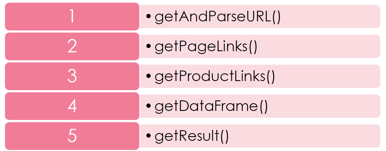 Figure 1 : Web Scraping Process
getAndParseURL()
Using this function, we can get the HTML code of the given URL to function.
getPageLinks()
Using this function, we recorded all page links to an empty list of products.
getProductLinks()
Using this function, we recorded all product links to an empty list for every page.
getDataFrame()
Using this function, we got pre-selected features for every product and recorded them to an empty list.
getResult()
Using this function, we created an entire dataframe from records and columns by giving the URL to the function.
So, if we call the getResult() function after defining all 5 functions, it returns an entire dataframe. Following is our data overview ;
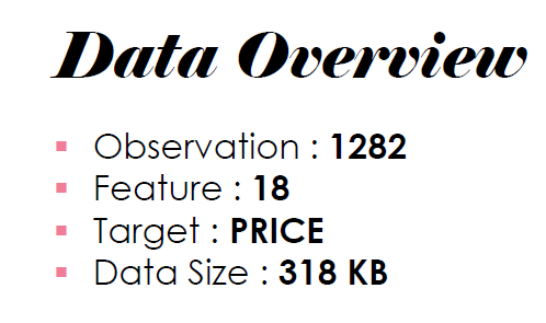 Figure 2: Scraped Data Overview
4. Data Cleaning and Transformation
After we scraped and transformed data into a dataframe, we made some transformations on columns such as taking only numeric from string values using split and replace functions like this.
Finally, we applied the following methods to handle “Missing” values ;
Filling with mode
Filling with mean
Filling with true-founded value
Dropping rows
As an example of “Missing” value handling code.
After data cleaning and transformation target variable’s distribution (PRICE) is as follows ;
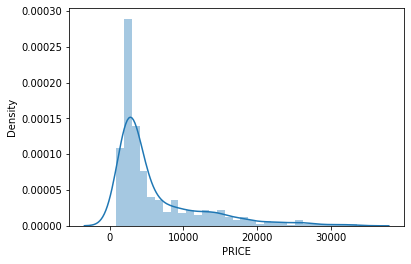 Figure 3: PRICE Distribution Plot
We decided that the product under 500 price value is outliers so filtered them. For a detailed process of data cleaning and transformation please click here.
5. Exploratory Data Analysis (EDA)
We visualized some features against to target variable which is PRICE to observe whether there is any linear relationship as follows ;
 Figure 4: RELEASE YEAR vs PRICE
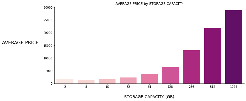 Figure 5: STORAGE CAPACITY vs PRICE
 Figure 6: RAM vs PRICE
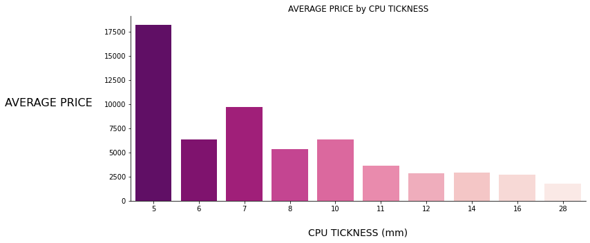 Figure 7: CPU THICKNESS vs PRICE
 Figure 8: SCREEN TECH vs PRICE
 Figure 9: CHARGE TYPE vs PRICE
As seen above bar charts, those 6 features have positive or negative linear or polynomial relationships with the target variable PRICE, also you can see the correlation heatmap given below ;
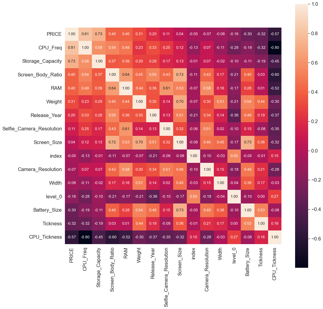 Figure 10: Correlation Heatmap
6. Feature Selection and Modeling
We sorted the dataset by product release year for testing the built model with the most up-to-date data. In the modeling process, we applied OneHotEncoding technique for the following features ;
Screen_Tech
CPU_Model
GPU_Model
Operating_System
Charge_Type
We used the following method in the model-building process ;
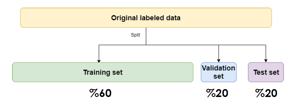 Figure 11: Train-Validation-Test Split
Given code shows us the building, predicting, evaluating, and K-Fold cross-validation process of a linear regression model with the train-validation-test split method.
7. Model Prediction and Interpreting Results
We used R2-Score and MSE as evaluation metrics in model prediction and made it for train-validation-test (%60-%20-%20)split,train-test(%80-%20) split and 10-Fold Cross-Validation.
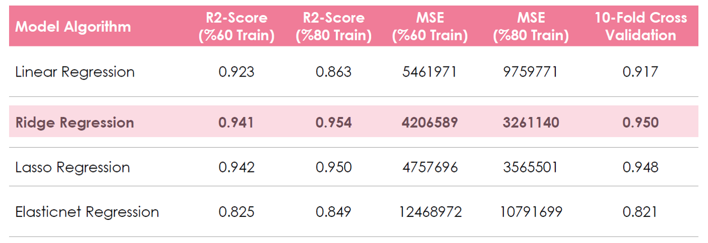 Figure 12: Model Prediction Results
As seen upper prediction result table, we did not expose overfitting or underfitting problems. To be able to avoid this problem, the most important part of a machine learning project is feature selection and data quality so we need to be careful at this stage. Finally, we selected Ridge Regression Model as it was the best one according to evaluation metrics.
8. Conclusion
This is the end of the article. In this article, I try to explain in detail the second project of our Data Science Bootcamp. As a reminder, you can visit the project’s GitHub repository from here. If you wish you can follow me on Medium.Hope to see you in my next article…
Appreciate the creator